The Gaussian beam is recognized as one of the most useful light sources. To describe the Gaussian beam, there is a mathematical formula called the paraxial Gaussian beam formula. Today, we’ll learn about this formula, including its limitations, by using the Electromagnetic Waves, Frequency Domain interface in the COMSOL Multiphysics® software. We’ll also provide further detail into a potential cause of error when utilizing this formula. In a later blog post, we’ll provide solutions to the limitations discussed here.
Gaussian Beam: The Most Useful Light Source and Its Formula
Because they can be focused to the smallest spot size of all electromagnetic beams, Gaussian beams can deliver the highest resolution for imaging, as well as the highest power density for a fixed incident power, which can be important in fields such as material processing. These qualities are why lasers are such attractive light sources. To obtain the tightest possible focus, most commercial lasers are designed to operate in the lowest transverse mode, called the Gaussian beam.
As such, it would be reasonable to want to simulate a Gaussian beam with the smallest spot size. There is a formula that predicts real Gaussian beams in experiments very well and is convenient to apply in simulation studies. However, there is a limitation attributed to using this formula. The limitation appears when you are trying to describe a Gaussian beam with a spot size near its wavelength. In other words, the formula becomes less accurate when trying to observe the most beneficial feature of the Gaussian beam in simulation. In a future blog post, we will discuss ways to simulate Gaussian beams more accurately; for the remainder of this post, we will focus exclusively on the paraxial Gaussian beam.
A schematic illustrating the converging, focusing, and diverging of a Gaussian beam.
Note: The term “Gaussian beam” can sometimes be used to describe a beam with a “Gaussian profile” or “Gaussian distribution”. When we use the term “Gaussian beam” here, it always means a “focusing” or “propagating” Gaussian beam, which includes the amplitude and the phase.
Deriving the Paraxial Gaussian Beam Formula
The paraxial Gaussian beam formula is an approximation to the Helmholtz equation derived from Maxwell’s equations. This is the first important element to note, while the other portions of our discussion will focus on how the formula is derived and what types of assumptions are made from it.
Because the laser beam is an electromagnetic beam, it satisfies the Maxwell equations. The time-harmonic assumption (the wave oscillates at a single frequency in time) changes the Maxwell equations to the frequency domain from the time domain, resulting in the monochromatic (single wavelength) Helmholtz equation. Assuming a certain polarization, it further reduces to a scalar Helmholtz equation, which is written in 2D for the out-of-plane electric field for simplicity:
where  for wavelength
  in vacuum.
The original idea of the paraxial Gaussian beam starts with approximating the scalar Helmholtz equation by factoring out the propagating factor and leaving the slowly varying function, i.e.,  , where the propagation axis is in
  and
and  is the slowly varying function. This will yield an identity
This factorization is reasonable for a wave in a laser cavity propagating along the optical axis. The next assumption is that  , which means that the envelope of the propagating wave is slow along the optical axis, and
  , which means that the variation of the wave in the optical axis is slower than that in the transverse axis. These assumptions derive an approximation to the Helmholtz equation, which is called the paraxial Helmholtz equation, i.e.,
The special solution to this paraxial Helmholtz equation gives the paraxial Gaussian beam formula. For a given waist radius  at the focus point, the slowly varying function is given by
\sqrt{\frac{w_0}{w(x)}}
\exp(-y^2/w(x)^2)
\exp(-iky^2/(2R(x)) + i\eta(x))
where  ,
,  , and
, and  are the beam radius as a function of , the radius of curvature of the wavefront, and the Gouy phase, respectively. The following definitions apply:
  ,
,  ,
,  , and
, and  .
.
Here,  is referred to as the Rayleigh range. Outside of the Rayleigh range, the Gaussian beam size becomes proportional to the distance from the focal point and the
  intensity position diverges at an approximate divergence angle of
  .
.
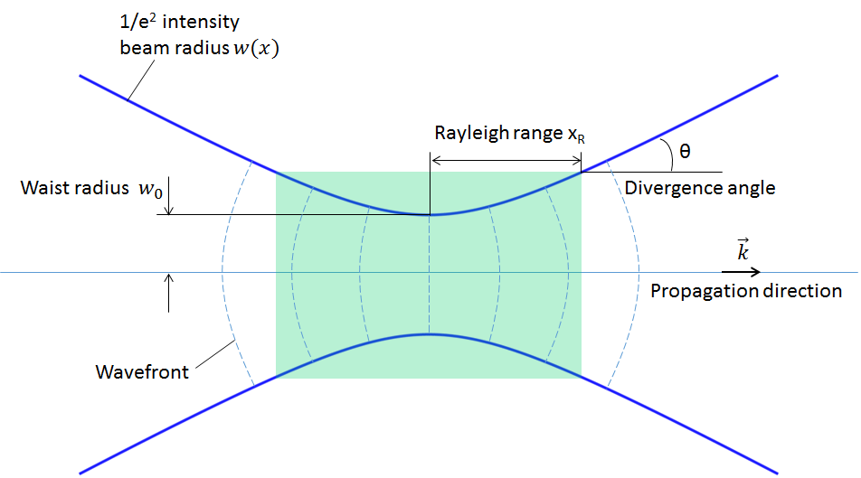
Definition of the paraxial Gaussian beam.
Note: It is important to be clear about which quantities are given and which ones are being calculated. To specify a paraxial Gaussian beam, either the waist radius
or the far-field divergence angle
must be given. These two quantities are dependent on each other through the approximate divergence angle equation. All other quantities and functions are derived from and defined by these quantities.
 must be given. These two quantities are dependent on each other through the approximate divergence angle equation. All other quantities and functions are derived from and defined by these quantities.
Simulating Paraxial Gaussian Beams in COMSOL Multiphysics®
In COMSOL Multiphysics, the paraxial Gaussian beam formula is included as a built-in background field in the Electromagnetic Waves, Frequency Domain interface in the RF and Wave Optics modules. The interface features a formulation option for solving electromagnetic scattering problems, which are the Full field and the Scattered field formulations.
The paraxial Gaussian beam option will be available if the scattered field formulation is chosen, as illustrated in the screenshot below. By using this feature, you can use the paraxial Gaussian beam formula in COMSOL Multiphysics without having to type out the relatively complicated formula. Instead, you simply need to specify the waist radius, focus position, polarization, and the wave number.

Screenshot of the settings for the Gaussian beam background field.
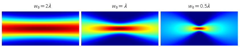
Plots showing the electric field norm of paraxial Gaussian beams with different waist radii. Note that the variable name for the background field is ewfd.Ebz.
Looking into the Limitation of the Paraxial Gaussian Beam Formula
In the scattered field formulation, the total field  is linearly decomposed into the background field
  and the scattered field
  as
as  . Since the total field must satisfy the Helmholtz equation, it follows that
  , where
  is the Laplace operator. This is the full field formulation, where COMSOL Multiphysics solves for the total field. On the other hand, this formulation can be rewritten in the form of an inhomogeneous Helmholtz equation as
The above equation is the scattered field formulation, where COMSOL Multiphysics solves for the scattered field. This formulation can be viewed as a scattering problem with a scattering potential, which appears in the right-hand side. It is easy to understand that the scattered field will be zero if the background field satisfies the Helmholtz equation (under an approximate Sommerfeld radiation condition, such as an absorbing boundary condition) because the right-hand side is zero, aside from the numerical errors. If the background field doesn’t satisfy the Helmholtz equation, the right-hand side may leave some nonzero value, in which case the scattered field may be nonzero. This field can be regarded as an error of the background field. In other words, under certain conditions, you can qualify and quantify exactly how and by how much your background field satisfies the Helmholtz equation. Let’s now take a look at the scattered field for the example shown in the previous simulations.
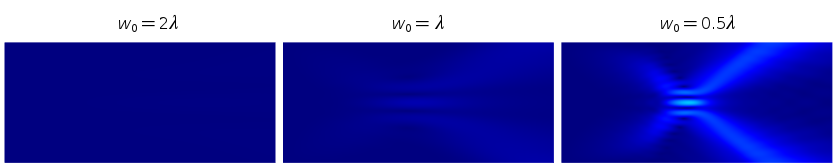
Plots showing the electric field norm of the scattered field. Note that the variable name for the scattered field is ewfd.relEz. Also note that the numerical error is contained in this error field as well as the formula’s error.
The results shown above clearly indicate that the paraxial Gaussian beam formula starts failing to be consistent with the Helmholtz equation as it’s focused more tightly. Quantitatively, the plot below may illustrate the trend more clearly. Here, the relative L2 error is defined by  , where
  stands for the computational domain, which is compared to the mesh size. As this plot suggests, we can’t expect that the paraxial Gaussian beam formula for spot sizes near or smaller than the wavelength is representative of what really happens in experiments or the behavior of real electromagnetic Gaussian beams. In the settings of the paraxial Gaussian beam formula in COMSOL Multiphysics, the default waist radius is ten times the wavelength, which is safe enough to be consistent with the Helmholtz equation. It is, however, not a “cut-off” number, as the approximation assumption is continuous. It’s up to you to decide when you need to be cautious in your use of this approximate formula.
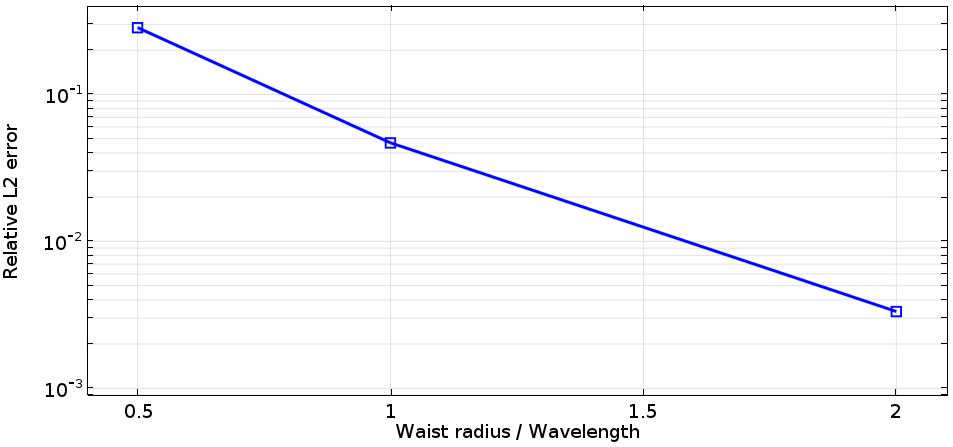
Semi-log plot comparing the relative L2 error of the scattered field with the waist size in the units of wavelength.
Checking the Validity of the Paraxial Approximation
In the above plot, we saw the relationship between the waist size and the accuracy of the paraxial approximation. Now we can check the assumptions that were discussed earlier. One of the assumptions to derive the paraxial Helmholtz equation is that the envelope function varies relatively slowly in the propagation axis, i.e., . Let’s check this condition on the x-axis. To that end, we can calculate a quantity representing the paraxiality. As the paraxial Helmholtz equation is a complex equation, let’s take a look at the real part of this quantity,  .
.
The following plot is the result of the calculation as a function of x normalized by the wavelength. (You can type it in the plot settings by using the derivative operand like d(d(A,x),x) and d(A,x), and so on.) We can see that the paraxiality condition breaks down as the waist size gets close to the wavelength. This plot indicates that the beam envelope is no longer a slowly varying one around the focus as the beam becomes fast. A different approach for seeing the same trend is shown in our Suggested Reading section.
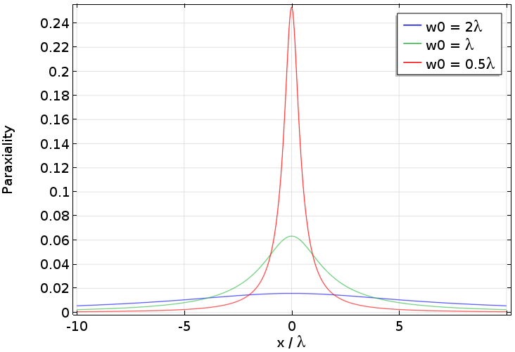
Real part of the paraxiality along the x-axis for paraxial Gaussian beams with different waist sizes.
Concluding Remarks on the Paraxial Gaussian Beam Formula
Today’s blog post has covered the fundamentals related to the paraxial Gaussian beam formula. Understanding how to effectively utilize this useful formulation requires knowledge of its limitation as well as how to determine its accuracy, both of which are elements that we have highlighted here.
There are additional approaches available for simulating the Gaussian beam in a more rigorous manner, allowing you to push through the limit of the smallest spot size. We will discuss this topic in a future blog post. Stay tuned!
Suggested Reading
- P. Vaveliuk, “Limits of the paraxial approximation in laser beams”, Optics Letters, Vol. 32, No. 8 (2007)
- Browse related topics here on the COMSOL Blog: